Measuring jitter accurately

With an accurate and clear picture of jitter performance, the test engineer can better understand jitter characteristics in the network or network device.
By Jim Anuskiewicz, Spirent Communications
Understanding latency characteristics in networks and devices has become even more critical thanks to the increase in delay-sensitive voice and video traffic over IP and Ethernet networks. Two key statistics should be measured when characterizing the temporal performance of a network: latency and jitter. Too much latency renders interactive applications such as voice and two-way video unusable, as the typical person will not tolerate excessive delays in conversation.
Similarly, excessive jitter makes the service unusable by negatively impacting service quality.
Jitter is the change in latency from packet to packet. RFC 4689 defines jitter as the absolute value of the difference between the forwarding delay of two consecutive received packets belonging to the same stream.
Applications and end-user devices are designed to tolerate a certain amount of jitter. This is achieved by buffering the data flow and designing processing algorithms to compensate for small changes in latency occurring from packet to packet.
Excessive jitter could cause the buffers to overflow, underflow, or even cause the algorithm to break down, resulting in dropouts in an audio stream or a choppy video display. Depending on the application, the tolerable amount of jitter will vary; however, it should usually be less than 50 msec for most triple-play services. A good service, for example, would have a jitter of 20 msec or less.
End-to-end network jitter (or service jitter) can be introduced in a variety of different ways such as when packets (in a flow) take different routes as a result of network congestion or link failure.
The more important cause of jitter, though, is introduced by network devices. Buffering, queuing, and switching architectures of any network device inherently have jitter. The jitter varies with traffic characteristics (packet burst distribution, packet length, traffic priority), traffic load, number of users, device load, etc. As traffic traverses a network, jitter is compounded by each device through which that traffic passes.
When designing a network or a network service, an accurate measurement of jitter should be available to quantify the jitter amount introduced by network components such as routers and switches. High-performance devices (high performance = low jitter) in the network reduce cumulative jitter and therefore provide high quality of service to users.
Three ways to measure jitter
Taking into account RFC 4689, the calculation of jitter requires measurement of the following four parameters:
- Transmit time of the first packet in the pair.
- Receive time of the first packet in the pair.
- Transmit time of the second packet in the pair.
- Receive time of the second packet in the pair.
Three common methods of measuring jitter are inter-arrival histogram; capture and post-process; and true, real-time jitter measurement.
Hardware required for jitter measurement varies based on the jitter measurement method used, the data rate to be analyzed, and the desired measurement accuracy. Slow traffic can be analyzed using a PC and the capture and post process method, but that only provides coarse accuracy. The best resolution that can be achieved with a PC is about 1 msec.
By contrast, true, real-time jitter measurement at high resolution requires specialized hardware to accurately processes the data in real time at line rates up to 10 Gbits/sec. High performance test equipment today achieves sub-100-nsec accuracy.
This article examines the advantages and limitations of the aforementioned three measurement methods. Other methods are not considered because they are insufficient for laboratory test environments. For example, jitter can be approximated as the difference between the maximum packet latency and minimum packet latency over a given period of time. However, this method fails to measure packet pair latency. Moreover, the results can be corrupted by macro changes in latency. For instance, the latency through a device could steadily increase from 20 msec to 200 msec over the period of the test. In this case, jitter would be calculated at 180 msec, which would be far higher than the actual packet-to-packet jitter.
A typical test plan for a network or network device would include a measurement for jitter performance under various traffic scenarios, including:
- Sending traffic at a constant rate (10%, 50%, 100%) using fixed length packets.
- Sending traffic at a constant rate using varying length packets.
- Sending traffic at a varying rate using varying length packets (realistic bursty traffic).
- Sending traffic-pair configuration without congestion.
The jitter measurement method should be evaluated against test scenario and traffic requirements.
Inter-arrival histogram method
A popular way to measure jitter, the inter-arrival method relies on packets transmitted at a known constant interval. With this method, two of the four needed parameters are pre-determined. Since packets are transmitted at a known fixed interval, only the inter-arrival time of the received packets is measured. The difference in the inter-arrival time between packets is the packet-to-packet jitter. Inter-arrival values are measured over a period of time and displayed in a histogram (see Fig. 1).

The inter-arrival method has one critical limitation and a few accuracy flaws. The limitation is that packets must be sent at equal intervals, which restricts measurement to only constant periodic traffic with fixed packet intervals. Depending on the complexity of the hardware generating traffic, there may be an additional restriction: fixed packet sizes. If the hardware can vary packet size but maintain an exact packet-to-packet interval, then varying packet sizes can be used. Because packets must be sent in perfectly equal intervals, it becomes impossible to measure jitter on traffic with a varying rate (bursty traffic).
A key accuracy flaw of the inter-arrival histogram method occurs when a packet is lost (i.e., dropped or corrupted). The inter-arrival time between the two packets before and after the dropped packet will be large and will corrupt the inter-arrival histogram. To eliminate corruption of results, inter-arrival measurements should be discarded when packet loss occurs. However, only the most advanced test equipment is capable of discarding the dropped packet inter-arrival data.
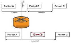
In the histogram in Fig. 2, for example, packet B was dropped (indicated by the red X) and did not arrive at the destination.
The inter-arrival time between Packet A and the next packet received (Packet C) was therefore calculated incorrectly since this method does not properly account for the lost packet (Packet B). The inter-arrival method will indicate an erroneously high jitter value due to these dropped packets.
The inter-arrival histogram method also fails to take into account packets arriving out of order. Packets arriving in a different order from the order in which they were sent also corrupt the measurement.
Capture and post-process method
A second common method for measuring jitter is to capture all packets and then process the data offline. Most test equipment puts a signature in the sent packets; thus, the capture file contains all the needed information (i.e., timestamps in the packets indicating Tx times and capture buffer hardware indicating Rx times). Test signatures also include packet sequencing information, making it possible to compensate for lost or out-of-sequence packets when using this method.
The critical limitation of the capture method is finite space in the buffer. The buffer can be filled up very quickly if data is sent at high speed. Typical test plans dictate the need to measure jitter over a much longer period of time than is possible with the largest capture buffers on most of the current test equipment. Another limitation of the capture method is the lack of real-time, cause-and-effect analysis. Debugging and analysis time is greatly reduced if the engineer can change a traffic load or device configuration parameter and see feedback in the jitter measurement. This real-time operation is not possible using the capture method.
True, real-time jitter measurement method
To provide a set of industry standard definitions, the Metro Ethernet Forum (MEF) released the MEF 10 specification in 2004, which contains a section defining the proper way to measure jitter while taking into account lost or corrupt packets. The flow chart in Fig. 3 illustrates how high-performance test offerings such as Spirent TestCenter 2.0 implement the MEF 10 jitter measurement definition.
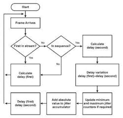
If the received packet is the first packet in the stream, then the packet transfer delay (latency) is calculated and stored.
If the received packet is not the first packet in the stream, then a check needs to be performed to make sure the packet is in the correct sequence. If the packet is not in sequence, latency results are discarded, and this packet is treated as the "new" first packet in the stream. This stops measurement corruption caused by lost or out-of-sequence packets.
If the received packet is the first packet and is in sequence, then the delay is calculated and stored. Next, the delay variation (jitter) is calculated by taking the difference of the delay of the current packet and the delay of the previous packet. Maximum, minimum, and accumulated jitter values are updated and stored. Finally, delay of the current packet is saved (to be used as the previous packet delay when the next packet arrives).
There are several advantages to true, real-time jitter measurement. First, packets do not need to be set at a known interval.
Second, the method can measure jitter on variable rate (bursty) traffic. Third, this method does not restrict test duration because the calculation occurs in real time as packets are received with no need of packet capture. Finally, real-time jitter measurement compensates for lost and out-of-sequence packets while producing results in real-time for instant feedback�even when varying traffic or device parameters.
Other advantages of true real-time jitter measurement include complex analysis views such as jitter charts or jitter histograms. These views produce far more revealing pictures than other measurement methods and substantially reduce test and analysis time. For example, the typical inter-arrival method produces a histogram of inter-arrival times showing how many packets were received in each inter-arrival bucket. When using only the inter-arrival histogram, it is not possible to determine when, where, or why abnormal amounts of jitter occurred. All that can be determined is the approximate maximum, minimum, and average jitter.

The table summarizes the key requirements for measuring jitter. Analyzing this table, it is evident that true real-time jitter measurement is superior to the other two methods. Real-time jitter measurement provides test scenario flexibility, accurate results, and real-time analysis capability. With an accurate and clear picture of jitter performance, the test engineer can better understand jitter characteristics in the network or network device.
Jim Anuskiewiczis a field systems engineering manager at Spirent Communications and heads its field engineering group covering the Spirent TestCenter performance analysis test system. He may be reached via the company's web site atwww.spirentcom.com.